2 Assignment 1 - NYC Shooting Insights

Author

Shannon Joyce

2.1 Introduction

I have been tasked with cleaning and analyzing NYC shooting data from the past 19 years. Using Tidyverse, I created insights to understand who the most common perpetrators and victims are, the frequency of and deaths from shootings over the years, as well as table summaries about the shootings.

library(tidyverse)
library(lubridate)
library(stringr)
library(tidyr)
library(ggplot2)
library(httr)
library(knitr)
library(readr)

2.2 Loading the Dataset

shooting_data <- read_csv("NYPD_Shooting_Incident_Data__Historic__20250910 (1).csv")

shooting_data %>% head(n=5) %>% kable()

Table 2.1: NYC Shooting Incident Data (first 5 rows).

INCIDENT_KEY	OCCUR_DATE	OCCUR_TIME	BORO	LOC_OF_OCCUR_DESC	PRECINCT	LOC_CLASSFCTN_DESC	LOCATION_DESC	STATISTICAL_MURDER_FLAG	PERP_AGE_GROUP	PERP_SEX	PERP_RACE	VIC_AGE_GROUP	VIC_SEX	VIC_RACE	X_COORD_CD	Y_COORD_CD	Latitude	Longitude	Lon_Lat
231974218	08/09/2021	01:06:00	BRONX	NA	40	NA	NA	FALSE	NA	NA	NA	18-24	M	BLACK	1006343.0	234270.0	40.80967	-73.92019	POINT (-73.92019278899994 40.80967347200004)
177934247	04/07/2018	19:48:00	BROOKLYN	NA	79	NA	NA	TRUE	25-44	M	WHITE HISPANIC	25-44	M	BLACK	1000082.9	189064.7	40.68561	-73.94291	POINT (-73.94291302299996 40.685609672000055)
255028563	12/02/2022	22:57:00	BRONX	OUTSIDE	47	STREET	GROCERY/BODEGA	FALSE	(null)	(null)	(null)	25-44	M	BLACK	1020691.0	257125.0	40.87235	-73.86823	POINT (-73.868233 40.872349)
25384540	11/19/2006	01:50:00	BROOKLYN	NA	66	NA	PVT HOUSE	TRUE	UNKNOWN	U	UNKNOWN	18-24	M	BLACK	985107.3	173349.8	40.64249	-73.99691	POINT (-73.99691224999998 40.642489932000046)
72616285	05/09/2010	01:58:00	BRONX	NA	46	NA	MULTI DWELL - APT BUILD	TRUE	25-44	M	BLACK	<18	F	BLACK	1009853.5	247502.6	40.84598	-73.90746	POINT (-73.90746098599993 40.84598358900007)

This code allowed me to upload this dataset from my computer into R. Now, I can start working with it.

Change in Data Source

This assignment was originally created by using an API to pull this public dataset directly from NYCOpenData (https://opendata.cityofnewyork.us/). This dataset has since been removed from their website, and a previously downloaded version of this dataset has been applied to this R script instead.

2.3 Data Cleaning

shooting_data_new <- shooting_data %>%
  mutate(
    PERP_AGE_GROUP = na_if(
      PERP_AGE_GROUP, "(null)"
      )
    )
shooting_data_new <- shooting_data_new %>%
  mutate(
     LOCATION_DESC= na_if(
      LOCATION_DESC, "(null)"
      )
    )
shooting_data_new <- shooting_data_new %>%
  mutate(
    PERP_SEX = na_if(
      PERP_SEX, "(null)"
      )
    )
shooting_data_new <- shooting_data_new %>%
  mutate(
    PERP_RACE = na_if(
      PERP_RACE, "(null)"
      )
    )

sum(is.na(
  shooting_data_new$PERP_AGE_GROUP)
  )

[1] 10972

shooting_data_new <- shooting_data_new %>% select(1:16)
shooting_data_2 <- shooting_data_new %>% filter(!is.na(PERP_AGE_GROUP))

First, I changed all (null) values and made them NA, that way they can be recognized when removing all rows that had NA values. I removed all NA values from the column perp_age_group in order to filter out rows that we don’t have enough information on.

shooting_data_2 <- shooting_data_2 %>% separate(
  col = OCCUR_TIME,
  into = c("Hour","Minute","Second"),
  sep = ":",
)

shooting_data_2 <- shooting_data_2 %>% mutate(Hour = as.numeric(Hour))
#and now...
shooting_data_2 <- shooting_data_2 %>%
  mutate(
    time_of_day = case_when(
      Hour >= 3 & Hour < 12  ~ "Morning",
      Hour >= 12 & Hour < 18 ~ "Afternoon",
      Hour >= 18 | Hour < 3 ~ "Night"
    )
  )

shooting_data_clean <- shooting_data_2 %>% select(1:19)

Next, I broke up the occur_time column into Hour, Minute, and Second columns. I used the Hour column to create a time_of_day column that specifies whether the shooting happened in the morning, afternoon, or night.

shooting_data_clean <- shooting_data_clean %>% separate(
  col = OCCUR_DATE,
  into = c("Year","Month","Day"),
  sep = "/",
)
shooting_data_clean$Day <- sub("T.*", "", shooting_data_clean$Day)

Finally, I had to break up the occur_date column into Month, Day, and Year columns in order to run some of the insights and graphs that I plan on doing.

2.4 Insights

2.4.1 Insight 1

shooting_data_clean %>% count(PERP_SEX) %>% kable()

Table 2.2: Table representing the total count of perpetrators from each sex. F = Female, M = Male, and U = Unknown.

PERP_SEX	n
F	461
M	16845
U	1466

This table shows us that almost four times the amount of shootings have been committed by men compared to women.

2.4.2 Insight 2

shooting_data_clean %>% count(PERP_SEX,VIC_SEX) %>% arrange(desc(n)) %>% kable()

Table 2.3: Table representing the total count of perpetrator sex/victim sex combinations. F = Female, M = Male, and U = Unknown.

PERP_SEX	VIC_SEX	n
M	M	15008
M	F	1830
U	M	1353
F	M	380
U	F	112
F	F	80
M	U	7
F	U	1
U	U	1

In the last 19 years, males have been the most common perpetrators as well as the most common victims. Female perpetrators have shot male victims more than they shot female victims.

2.5 Tables and Graphs

2.5.1 Graph 1

shooting_by_time_of_day <- shooting_data_clean %>% 
  group_by(time_of_day) %>% 
  dplyr::summarize(total = n())

ggplot(shooting_by_time_of_day, aes(x = time_of_day, y = total)) +
  geom_bar(stat = 'identity', fill = 'steelblue') +
  labs(title = "Frequency of Shootings in NYC by Time of Day",
       x = "Time of Day",
       y =" Total" +
         theme(
           plot.title = element_text(size=15, family = "serif", face = "bold")
         )
  )

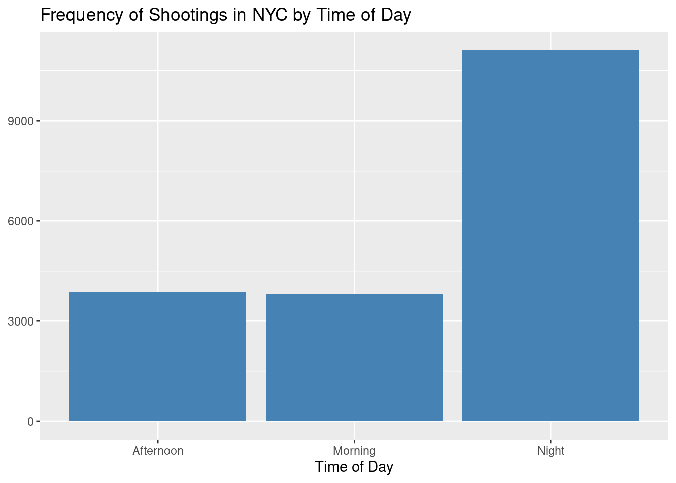
Figure 2.1: Total number of shootings in NYC grouped by morning, afternoon, and night.

This graph shows us that most shootings occur at night.

2.5.2 Table 1

murders_per_year <- shooting_data_clean %>% 
  filter(STATISTICAL_MURDER_FLAG == TRUE) %>%
  group_by(Year)
murders_summary <- murders_per_year %>% 
  count(Year,STATISTICAL_MURDER_FLAG)

murders_summary <- murders_summary %>% rename(total = n)

murders_summary %>% select(1,3) %>% kable(caption = "Gun Murders per Year, NYC: 2006-2024")

Table 2.4: Total count of shootings that resulted in death each year from 2006-2024.

Gun Murders per Year, NYC: 2006-2024
Year	total
01	266
02	231
03	257
04	314
05	414
06	353
07	404
08	359
09	382
10	299
11	244
12	305

2.5.3 Graph 2

ggplot(murders_summary, aes(x = Year, y = total, group = 1))+
  geom_line(color = 'red', linewidth = 1) +
  labs(title = "Gun Murders in NYC per Year",
       x = "Year",
       y =" Murders by Gun") +
  theme(
    plot.title = element_text(size=20, family = "serif", face = "bold")
  )

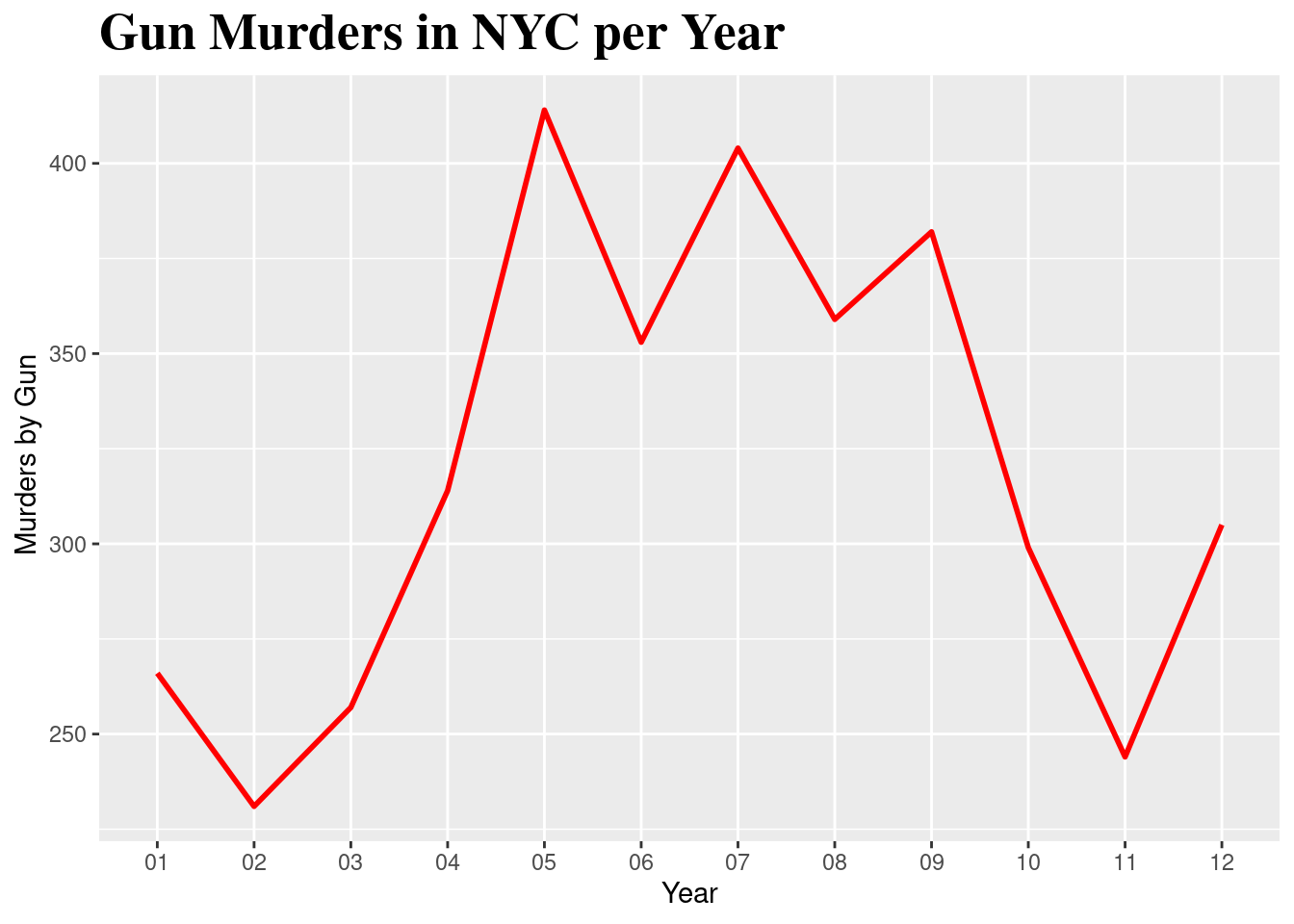
Figure 2.2: Total number of shootings that have resulted in death each year since 2006.

This graph shows us the trend line of how many shootings resulted in murder each year from 2006-2024. There had been a steady decline with a spike in 2020.

The average amount of shootings that result in death in NYC each year is 319 per year.

2.6 Reflection

I could see this workflow helping me in my thesis research because it seems to be a good tool for creating a coherent and comprehensive document to look back on and follow. Additionally, it seems easy to share my thought process/analyses with my mentor, and an accessible way for her to collaborate on my code if need be. While I still have to figure out the best way to utilize this kind of workflow, I can definitely see it having benefits to keep everything organized for myself and my data, and for reproducibility purposes.